3 × 3 m satellite imagery makes sense in agriculture, but it is not an automatic answer to every problem related to crop monitoring and variable rate application. It delivers the greatest value when image resolution matches the scale of the agronomic decision, field variability, the farm’s budget and the real capabilities of the machine.
Satellite image resolution in agriculture is a remote sensing data parameter that defines how small a part of the field is represented by a single pixel and how effectively that image can be translated into an agronomic decision, an application map, crop scouting or risk analysis.
In brief
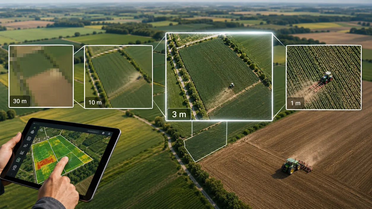
High-resolution satellite imagery helps detect field variability more accurately, but on its own it does not guarantee better VRA. In practice, resolution must be matched to the decision: 250–1,000 m for regional analysis, 30 m for historical data and broad trends, 10 m for farm-level monitoring, 3 m for zones and anomalies, 1 m and 30–50 cm for detailed diagnostics, and drones for assessing rows, plant population and localised damage.
- Sentinel-2 10 m is still sufficient for many applications in field crops.
- Landsat 30 m has strong historical value, but is too coarse for most VRA decisions on small fields.
- PlanetScope at around 3 m is particularly useful for small fields, soil mosaics, vegetables, orchards and anomalies.
- 1–1.5 m imagery makes sense where infrastructure, plots, rows or the boundaries of a problem need to be seen more clearly.
- 30–50 cm imagery and drones do not replace VRA across the whole farm. They are primarily diagnostic tools.
- The cost of data increases with resolution, number of acquisitions, image freshness, order area and processing level.
- System performance decreases when the number of pixels grows faster than the value of the decision. This is a common mistake.

Are 3 × 3 m satellite images really needed?
3 × 3 m satellite images are needed when the agronomic decision concerns small zones, irregular fields, high-value crops or strong site variability. They are not needed when the farm applies treatments uniformly anyway and the machine does not support variable rate application.
As of May 2026, agricultural technology offers often use a simple argument: 3 m is “better” than 10 m. That is an oversimplification. A 10 × 10 m pixel represents 100 m², while a 3 × 3 m pixel represents 9 m², but in practice the question is not only: “what can be seen?”. The question is: “what decision can be made from it?”.
Sentinel-2 has 13 spectral bands, including 4 bands at 10 m resolution, 6 bands at 20 m and 3 bands at 60 m, while its imaging swath is 290 km according to the Copernicus Data Space Ecosystem. The Sentinel-2 specification in Copernicus Data Space shows that this is not a “coarse image”, but a fully fledged source of multispectral data for crop monitoring.
PlanetScope provides imagery at around 3 m with frequent coverage, which increases the chances of capturing a field at the right time and without cloud cover. Data of this class is highly useful for zoning, detecting soil mosaics and checking anomalies, but it does not replace soil testing, yield maps, crop scouting or knowledge of field history. In short: 3 m is a tool, not a strategy.
The biggest mistake is comparing resolutions without asking what they will be used for. A 30 cm image may be excellent for checking damage, infrastructure or the boundary of a flooded area, while at the same time being too expensive and operationally too heavy for weekly monitoring of 2,000 ha of cereals. Sentinel-2, meanwhile, may be too coarse for strawberry rows, but very good for observing crop canopy condition on a large farm.
What does satellite image resolution mean in agriculture?
Satellite image resolution does not only mean pixel size. In agricultural practice, spatial, spectral, temporal, radiometric and operational resolution must all be assessed. Operational resolution means the ability to translate the image into a decision, an application file, a field operation and subsequent documentation.
Spatial resolution indicates how large an area of the field is averaged into a single pixel. A 3 m pixel does not show an individual plant. It shows a signal from 9 m², which may combine crops, soil, weeds, tramlines, shadows and harvest residues.
Spectral resolution is just as important. In agriculture, an attractive RGB image is not enough, because crop condition analysis is based on the red band, near-infrared, red edge and sometimes SWIR. This is why a very sharp panchromatic image is not always agronomically better than a lower-resolution multispectral image.
Pléiades Neo has a resolution of 30 cm in the panchromatic band and around 1.2 m in multispectral mode. This is a good example of the trade-off: an image may be visually very sharp, but for vegetation indices it is still necessary to check which bands are available and at what resolution.
Temporal resolution determines whether the image is available when a decision needs to be made. ESA describes Sentinel-2 as a mission with 13 bands, 10 m resolution in selected bands, a 290 km swath and a 5-day revisit time for the constellation. This matters because, during intensive crop growth, image freshness can be more important than pixel size alone.
Operational resolution is most often overlooked. It means the minimum scale at which the farm, advisor and machine can respond meaningfully. If a spreader works at 24 m and the decision is to be executed in 30–50 m zones, a 30 cm image may not improve the quality of the application map, even if it looks far more detailed.
Which image resolutions make sense in agriculture?
Every resolution class has its place. The larger the pixel, the better it is for regional scale, historical analysis and unit cost. The smaller the pixel, the better the local diagnostics, but the higher the cost, the larger the data volume and the greater the risk that the analysis becomes more precise than the decision itself.
| Resolution | Typical sources | When it makes sense | When it does not make sense | Practical conclusion |
|---|---|---|---|---|
| 250–1,000 m | MODIS, Sentinel-3 | Regional drought, national monitoring, weather and vegetation trends, macro models for agri-food | Individual fields, VRA, small farms, operational decisions | Good for regional analytics, weak for the farmer in the field. |
| 30 m | Landsat 8/9 | Field history, multi-year analysis, large areas, moisture and land surface temperature trends | Small plots, soil mosaics, precise zones, section-based operations | Historical value is greater than current operational precision. |
| 10 m | Sentinel-2 | Seasonal monitoring, NDVI, NDRE, large fields, basic management zones | Rows, small blocks, orchards, vegetables, boundaries of small damage areas | The best free baseline for most field crop farms. |
| 3–5 m | PlanetScope, SPOT, selected commercial data | Small fields, mosaics, vegetables, zoning, anomalies, frequent observations | Uniform fields, no VRA, no ground validation, no decision-making process | A good premium layer for diagnostics and zones. |
| 1–1.5 m | SPOT 6/7, Pléiades multispectral, selected VHR data | Plots, infrastructure, larger rows, orchards, damage, problem boundaries | Weekly monitoring of low-value large-scale crops | Useful where the cost of error is high. |
| 30–50 cm | SkySat, Pléiades Neo, Maxar, other VHR sources | Damage, audits, infrastructure, precise boundaries, high-value crops | Mass VRA for cereals if the machine and agronomy do not work at this scale | A control and diagnostic tool, less often a day-to-day crop monitoring tool. |
| 2–20 cm | RGB drone, multispectral drone, machine-mounted camera | Plant population, weeds, rows, localised damage, diseases, plantation assessment | Large areas without organised flights and processing | Best for detailed diagnostics, not always for a 1,000 ha scale. |
| 5–20 m radar | Sentinel-1 SAR, selected commercial SAR data | Clouds, surface moisture, canopy structure, flooding, monitoring independent of light | Simple visual interpretation like NDVI, without a model and calibration | Radar is highly useful, but requires different interpretation from optical imagery. |
Source: FarmPortal’s own analysis based on public specifications from Copernicus, USGS, NASA Earthdata, Planet, Airbus and practical EO data processing for agriculture.
When does 250–1,000 m make sense?
A resolution of 250–1,000 m is not suitable for decisions on an individual field, but it does make sense in regional analysis. MODIS and Sentinel-3 can support drought monitoring, vegetation anomalies, raw material supply risk, meteorological conditions and trend analysis at regional, national or supplier-portfolio level.
For a processor, distributor or trading company, this scale can be useful earlier than 30 cm imagery. If the aim is to answer whether a region producing onions, potatoes or apples is experiencing drought stress, a very high-resolution image is not needed. A regional signal combined with weather data and supplier information is enough.
When does 30 m make sense?
Landsat 30 m has lower spatial precision than Sentinel-2, but it is highly valuable historically. In practice, it can help assess long-term field trends, zone stability, drought history, land surface temperature and land-use changes. For current VRA in a fragmented farm, it is usually too coarse.
In Poland, 30 m easily combines different elements: part of a field, a field margin, shadow, a road, a pond or a neighbouring crop. Landsat should therefore be treated as a contextual and historical layer rather than the basis for a direct application map for small plots.
When does 10 m make sense?
Sentinel-2 10 m is most often the best starting point for field crop farms. The data is free, regular, multispectral and sufficient for monitoring most fields of several, several dozen or tens of hectares. It works particularly well for seasonal trends, field comparison and detecting large stress zones.
Limitations appear with small plots, irregular boundaries and row crops. If a plot is 1–2 ha, a 10 m pixel may cover too large a part of the field to safely distinguish small zones. This is where 3 m imagery or a drone begins to have a real justification.
When does 3–5 m make sense?
A resolution of 3–5 m is the strongest candidate for a premium agricultural layer. It shows more detail than Sentinel-2, while still being operationally easier than 30 cm imagery or a drone orthomosaic. This makes it suitable for zoning, anomaly checks, scouting plans and advisory work.
In this resolution class, frequency matters. A single highly detailed image taken after an unsuitable operation or a short dry spell can be misleading. A series of images taken at the right times makes it possible to distinguish a stable problem from a temporary weather effect.
When does 1–1.5 m make sense?
1–1.5 m imagery is useful in orchards, vegetables, potatoes, sugar beet, infrastructure and contract crops. It makes it easier to see plot boundaries, service roads, small flooded areas, damage, bare patches, gaps in the canopy and larger differences in rows. It is still not an image of an individual plant.
From a cost and operational perspective, this resolution should be used selectively. It does not always make sense to buy it for the entire farm. A mixed model is often better: Sentinel-2 as the baseline, 3 m for problematic fields, 1 m for selected plots and drones where the cause needs to be confirmed.
When does 30–50 cm make sense?
30–50 cm imagery is very strong for damage checks, audits, infrastructure, flood boundaries, insurance documentation, precise plot boundaries and high-value plantations. In field crop production, it should rarely be the first choice, because cost and data load rise quickly.
This resolution can be highly relevant for processors and insurers. It helps document an event, compare plantation condition, indicate the affected area and reduce disputes over the size of the problem. For nitrogen fertilisation of 300 ha of wheat, it will often be excessive.
When is a drone better than a satellite?
A drone is better when the decision concerns rows, plant population, individual disease outbreaks, weeds, lodging, frost damage, bare patches or detailed plantation documentation. Satellites win on regularity and scale, but drones win on resolution and control over flight timing.
The problem with drones starts at scale. Flights, operational permissions, weather, batteries, the operator, processing, orthorectification, mosaicking and data archiving create a real process cost. A drone is not a free “better satellite”. It is a separate operation.
When does radar make sense?
Radar, such as Sentinel-1 SAR, makes sense when clouds prevent optical observations or when the focus is on surface moisture, flooding, canopy structure, approximate biomass changes and signals independent of sunlight. It is not a simple replacement for NDVI.
In practice, radar works best as an additional layer. For the farmer, radar imagery is less intuitive than a vegetation index, but for analytical systems it can be very valuable, especially in wet seasons and regions with frequent cloud cover.
How much do different satellite image resolutions cost?
The cost of satellite imagery depends on resolution, provider, area, number of acquisitions, image freshness, cloud cover, processing level, licence and whether the purchase covers archive imagery, new tasking, seasonal monitoring or a ready-made analysis. This is why thinking in terms of “price per pixel” is the wrong approach.
The cheapest data is public data, such as Sentinel-2, Sentinel-1, Landsat, MODIS and Sentinel-3. The licence cost of the image is then PLN 0, but processing, cloud computing, validation, interpretation, FMS integration and recommendation preparation still need to be paid for. Free data does not mean a free decision.
Commercial data is usually priced differently. Sales platforms and brokers sometimes quote prices per km², but in practice there may be minimum order areas, subscriptions, packages, download limits, different prices for archive data and new tasking, and additional processing costs. For PlanetScope in agriculture, a subscription model linked to the monitored area is often used, rather than a simple one-off price for a single scene.
| Data class | Data cost | Typical purchase model | Hidden operational cost | When it makes economic sense |
|---|---|---|---|---|
| Sentinel-1, Sentinel-2, Landsat, MODIS, Sentinel-3 | PLN 0 for the public data licence | Public access, API, EO platforms, own processing | Cloud, algorithms, validation, agronomist’s work, integration | Continuous monitoring, large areas, FMS baseline, historical analysis |
| 3–5 m commercial | Usually a subscription or area-dependent quotation | Seasonal monitoring, area under management, purchase through a platform | Image selection, cloud masks, harmonisation with Sentinel-2, recommendations | Small fields, vegetables, advisory services, zones, frequent observations |
| 1–1.5 m | Usually higher than 3–5 m, often priced per km² or as a package | Archive, tasking, selected fields or plots | More pixels, larger transfer, more quality control | High-value crops, orchards, damage, infrastructure |
| 30–50 cm | Often several dozen USD/km² depending on source and acquisition mode | Archive, tasking, minimum area, rapid acquisition | Large files, manual interpretation, orthorectification, timing selection | Audit, damage, quality control, high-value plantations |
| Drone 2–20 cm | Service cost depends on area, equipment, operator and product | Contracted flight, own drone, periodic plantation inspection | Operator, batteries, weather, processing, archiving, flight time | Detailed diagnostics, rows, plant population, weeds, localised damage |
The difference between data cost and decision cost matters. 10 m data may be free, but a poorly prepared recommendation can cost more than a commercial image. 30 cm data may be expensive, but justified if it documents damage on a high-value plantation.
Why can price per hectare be misleading?
Farmers often want to know the price per hectare. This is understandable, but in remote sensing the cost does not always scale linearly. A provider may have a minimum order area, minimum transaction value, price per scene, price per km², seasonal price, API price or price based on the number of acquisitions.
The example is simple. An 80 ha farm may pay relatively a lot for a one-off 30 cm image if the minimum purchase area is 25 km². A 2,000 ha farm, meanwhile, may receive a better unit price in a 3 m subscription, but pay more for processing the entire season.
When is more expensive data cheaper in practice?
More expensive data can be cheaper if it shortens response time or reduces the number of unnecessary field inspections. For an advisor working with multiple farms, 3 m imagery can reduce the number of unnecessary field visits. For a processor, high-resolution imagery can accelerate the decision to inspect a supplier.
More expensive data does not make sense if it ends up as a coloured map without a decision. This is the key economic test: does the image change the rate, timing, scouting location, sampling plan, procurement plan or documentation? If not, the cost is difficult to defend.
How does resolution affect data processing performance?
The higher the resolution, the faster the number of pixels, data transfer, storage cost and analysis time increase. Moving from 10 m to 1 m does not mean 10 times more data. It means roughly 100 times more pixels for the same area.
| Resolution | Pixel area | Number of pixels per 100 ha | Impact on performance |
|---|---|---|---|
| 30 m | 900 m² | around 1,111 | Very light processing, but low field-level detail |
| 10 m | 100 m² | 10,000 | Good balance between scale and processing cost |
| 3 m | 9 m² | around 111,111 | Around 11 times more pixels than 10 m |
| 1 m | 1 m² | 1,000,000 | Around 100 times more pixels than 10 m |
| 50 cm | 0.25 m² | 4,000,000 | Heavy load for transfer, analysis and archiving |
| 10 cm from a drone | 0.01 m² | 100,000,000 | Very large files; good processing and data selection are necessary |
Source: FarmPortal’s own calculations for an area of 1 km². In practice, file size also depends on the number of bands, product type, compression, radiometric depth, metadata, format and number of acquisition dates.
Performance is not only about the server. It is also about the agronomist and the farmer. The more detailed the map, the more potential spots, boundaries and exceptions there are. If the system does not generalise data into meaningful zones, the user receives more detail but fewer decisions.
Why can 30 cm imagery make the process worse?
A 30 cm image can show tramlines, shadows, ruts, parts of plants, poles, trees, furrows and many small objects. This is valuable diagnostic information, but for a fertilisation map it may be noise. Not every detail should change the rate.
In a well-designed system, very high-resolution data is filtered. The goal is to extract stable agronomic information, not to transfer every pixel into the machine terminal. This is particularly important for fertilisation, drilling and section-controlled spraying.
How should performance be matched to the process?
For monitoring 2,000 ha every few days, a light, automated process based on Sentinel-2 and possibly 3 m imagery for selected fields will be better. For 20 ha of strawberries or contract vegetables, a heavier diagnostic process may be more cost-effective, because decisions are more frequent and the value per hectare is higher.
This is the difference between monitoring and inspection. Monitoring should be repeatable, low-cost and scalable. Inspection should be accurate, contextual and carried out when there is a specific problem.
How should resolution be matched to the crop and decision?
Resolution must be matched to the crop, production value, field size, soil variability and type of decision. Cereals on large fields often do not need 3 m imagery at every date, whereas vegetables, potatoes, sugar beet, orchards and soft fruit more often justify higher accuracy.
In large-scale crops such as wheat, maize, oilseed rape or soya, Sentinel-2 works well as a baseline layer. It helps observe the canopy, detect large stress zones, compare fields, plan scouting and build initial management maps. For many farms, this is enough.
3 m imagery makes more sense when the field is small, irregular or highly variable. In Poland, this is common. Plot fragmentation, soil mosaics, wedges, small woodland areas and varied fertilisation history mean that a 10 m pixel may mix zones with different yield potential.
In vegetables and potatoes, decisions are more frequent and the cost of error is higher. Water shortage, uneven emergence, plant population issues or disease stress can quickly affect marketable quality. Here, 3 m imagery is often a sensible screening layer, but analysis of rows, weeds and individual disease outbreaks usually requires a drone, field inspection or machine-mounted camera.
Orchards, soft fruit and vineyards are even more demanding. A 10 m pixel combines tree crowns, inter-rows, shade, soil, service tracks and structures. 3 m data helps locate problematic blocks, but decisions about pruning, spray volume or the condition of individual rows require data closer to the plant, such as LiDAR, multispectral cameras, ground measurements and precise scouting.
| Crop or system | Typical decision | Sufficient baseline | When to pay for higher resolution | When a drone or camera is needed |
|---|---|---|---|---|
| Cereals, oilseed rape, maize | Fertilisation zones, scouting, field comparison | Sentinel-2 10 m | Small fields, strong variability, irregular boundaries | Plant population assessment, weeds, localised damage |
| Potatoes and sugar beet | Irrigation, canopy condition, yield zones | 10 m or 3 m | Contracting, quality, short decision windows | Rows, gaps, diseases, detailed plant population |
| Field vegetables | Water, crop protection, variation between plots | 3 m | High value per ha and frequent treatments | Weeds, damage, inter-row analysis |
| Orchards, soft fruit, vineyards | Problem plots, stress, scouting plan | 3 m as screening | Plot monitoring, damage, audit, infrastructure | Canopies, rows, leaf wall volume, section-controlled spraying |
| Contract plantations | Supply risk, quality, harvest timing | 10 m and 3 m | When a supplier has high quality or logistical risk | Verification of damage, plant population or disease before harvest |
Source: FarmPortal’s own analysis based on Sentinel-2, PlanetScope and Pléiades Neo parameters and practical interpretation of satellite data for field crops and specialist crops.
Does 3 × 3 m make sense for VRA?
3 × 3 m imagery makes sense for Variable Rate Application (VRA) as input data for analysis, but it should rarely be the final application grid. Most often, it should be transformed into larger, stable zones that the machine can actually execute.
VRA does not mean that every pixel in the image automatically becomes a separate rate. Good VRA starts with identifying variability and ends with an operation performed by a spreader, sprayer, drill or planter. In between, noise must be removed, data layers combined, rates defined, a file prepared and terminal compatibility checked.
3 m data is very good for building management zones, selecting sampling locations, comparing with a yield map and locating anomalies. A 2021 study by Yuval Sadeh and co-authors described the fusion of Sentinel-2 and PlanetScope data for daily 3 m LAI estimates in wheat, compared with 57 in situ measurements in Australia and Israel. This demonstrates the value of high spatio-temporal resolution in crop analysis, but it does not mean that the rate should automatically change every 3 m.
If a spreader works at a width of 24–36 m, a 3 m pixel should help build 20–50 m zones rather than control the rate pixel by pixel. Similarly, in a sprayer with sections several metres wide, the map must account for section width, speed, valve response time and rate stability. Otherwise, the result is a map that looks good but is difficult to execute.
A useful practical sentence is simple: a 3 × 3 m image should act as a microscope for field diagnosis, not as a direct instruction for every nozzle, coulter or spreading disc.
Can agricultural machinery execute a map with 3 m accuracy?
Many modern machines support VRA, but this does not mean the operation is performed with accuracy equal to the satellite pixel. A machine executes a rate command that depends on the terminal, controller, GNSS, sections, working width, hydraulic or pneumatic delays and the type of material being applied.
The ISO 11783 standard, known in practice as ISOBUS, organises communication between the tractor, terminal and implement. TC-GEO handles location-based tasks, including variable rate application, while TC-SC handles automatic section switching. AEF also describes the use of ISO-XML for data exchange between a farm management system and the Task Controller. This is technically important because the map itself is not enough without a compatible data chain.
Variable rate technology can work in map-based or sensor-based mode. University of Florida IFAS Extension describes Variable Rate Technology as a system that changes the application of water, fertilisers or crop protection products in response to spatial variability in the field. The IFAS publication on VRT explains the distinction between map-based and sensor-based approaches.
| Operational limitation | Practical impact | How to reduce the risk |
|---|---|---|
| Working width of 24–36 m | Fine variability from a 3 m map may be impossible for the spreader to execute | Generalise pixels into stable management zones |
| Sprayer section width | The machine responds by sections, not by individual image pixels | Design the map around the actual section layout |
| Dosing delay | The rate changes with an offset relative to the GNSS position | Account for terminal calibration, speed and response time |
| GNSS accuracy | Position error can shift zone boundaries | Use corrections and RTK where the decision requires it |
| File format | Not every terminal supports the same file and rate structure | Export ISO-XML or SHP compatible with the terminal |
Source: FarmPortal / Agri Solutions’ own analysis based on the ISO 11783 standard, AEF materials and practical experience in preparing application maps for spreaders, sprayers, drills and planters, as well as internal research.
When is it worth paying for high resolution?
It is worth paying for high resolution when it leads to a decision that can be executed and measured. You do not pay for pixels themselves. You pay for better zones, more accurate scouting, lower risk of applying the wrong rate, earlier detection of a problem or better production documentation.
The economics of high resolution depend on field variability. In their 2021 paper on information accuracy in variable rate technologies, Späti, Huber and Finger described that the net benefits of more accurate data increase particularly in fields with greater heterogeneity of soil conditions and lower autocorrelation of soil types. This is a sober counterargument to the slogan “more pixels equals more profit”.
On a farm with large, uniform fields, a better first step may be to organise field boundaries, treatment history, soil tests and yield maps. On a vegetable, orchard or contract farm, 3 m imagery can provide a faster information return because decisions are more frequent and raw material quality carries greater financial weight.
There are also situations where 3 m does not make sense. If the farmer applies one rate across the whole field, has no compatible terminal, does not carry out scouting and does not validate the image with soil samples, the more expensive image will only be a better-looking map. Better-looking, but not necessarily useful.
When is 3 m a real need?
- The farm has small or irregular plots.
- The crop has high economic value per hectare.
- Soil variability is strong and frequent.
- Decisions are made at plot, zone or sub-field level.
- The map is combined with soil samples, yield, weather and scouting.
- The machine genuinely supports VRA.
- The final map is generalised into zones that can be executed.
When is 3 m just a trend?
- The customer wants a “better image” but does not specify the agronomic decision.
- The service ends with a coloured NDVI map without a recommendation.
- There is no ground data for validation.
- The machine does not perform variable application.
- The image resolution is higher than the practical precision of the field operation.
- The farm applies one rate across the whole field anyway.
When does higher resolution not pay back economically?
Higher resolution does not pay back when the cost of data, processing and service is greater than the value of the decision. For a large, uniform wheat field, buying 30 cm imagery just to generate NDVI is usually hard to justify. For a vegetable plantation, where a 2-day delay can affect marketable quality, the same cost may be rational.
The best cost model is a layered model: public data for all fields, 3 m for fields requiring greater accuracy, 1 m or 30–50 cm for selected cases, and a drone where the cause of the problem must be confirmed. This approach limits costs and avoids overloading the process.
Which data must be combined to make a VRA map reliable?
A reliable VRA map should not be based on a single satellite image. It requires a combination of satellite data, soil samples, fertilisation history, yield maps, scouting, weather, field boundaries, machine parameters and the agronomic objective.
A satellite image shows the condition of crops or the field surface at a specific moment. By itself, it does not say whether a problem is caused by nitrogen deficiency, soil compaction, pH, drought, disease, poor plant population, herbicide damage or drilling error. Without supporting data, the interpretation may be visually accurate but agronomically wrong.
Good practice is to treat the satellite as a screening layer. First, the image indicates zones; then an agronomist or farmer checks the cause in the field; only then is a recommendation created. In later seasons, maps should be compared with yield, treatment costs and soil analysis results, because stable variability has greater value than a one-off image taken after rainfall.
Minimum dataset for an application map
- current field boundaries and crops,
- treatment and fertilisation history,
- soil test results with GPS location,
- a satellite layer, such as NDVI, NDRE or LAI,
- scouting of problem zones,
- target rates and agronomic constraints,
- terminal and machine parameters,
- export format, such as ISO-XML or SHP.
Success metrics should be practical: number of hectares covered by a correct map, percentage of fields with soil validation, number of zones executed without terminal error, rate difference compared with a uniform-rate option, fertiliser cost per hectare, marketable yield, raw material quality and completeness of treatment documentation.
What do different user groups gain?
The value of high resolution is different for the farmer, advisor, processor, machinery manufacturer and R&D partner. Each group has a different problem: some want to execute a field operation, others want to confirm supply quality, sell an advisory service or check whether a technology works under field conditions.
The farmer needs a decision, not another map. For a 100–300 ha farm, fertiliser costs, fuel, services, operation timing and machine compatibility are what matter. The best first step is to organise fields, soil samples, treatment history and machinery data, and only then purchase premium layers.
The agricultural advisor uses 3 m imagery as a tool for prioritising work. Instead of visiting all fields one by one, the advisor can identify plots or zones that require scouting. This changes the way work is done: less guessing, more discussion about the cause of the problem.
A fruit and vegetable processor looks at the data more broadly. For them, satellite data can support supplier monitoring, quality risk assessment, identification of plantations that are delayed or under water stress, and procurement planning. It will not replace raw material quality control, but it can reduce the number of surprises before harvest.
A machinery manufacturer should look at high resolution through the lens of compatibility. If the terminal, controller and implement cannot receive the map, the farmer will not feel the value of the data. This is why integration with ISOBUS, TC-GEO, TC-SC, ISO-XML, SHP and telematics is part of the product, not a marketing add-on.
An R&D partner can use 3 m imagery to validate hypotheses, build models and plan experiments. The methodology, however, matters: control field, georeferencing, ground measurements, seasonal repeatability and a clearly defined KPI. Without this, a project can easily produce maps, but not knowledge.
How does FarmPortal support work with satellite data?
FarmPortal supports work with satellite data when the image is part of a process: from field, through observation and recommendation, to application map, treatment, documentation and cost analysis. This is what separates crop monitoring from merely viewing indices.
In practice, the user needs one environment where fields, crops, treatments, GPS notes, scouting photos, weather data, soil samples and production history are visible. This setup makes it possible to interpret NDVI or NDRE together with what actually happened in the field. A full overview of modules is available on the FarmPortal farm management functions page.
FarmPortal acts as a data and integration layer. It can combine data from FMS, IoT sensors, weather stations, GPS devices, machine telematics, ERP systems and analytical tools. For VRA, it is particularly important that the map is not a detached file, but part of a process that can be planned, executed and accounted for.
For those developing a variable rate process, the FarmPortal article on practical implementation of VRA is also useful. It complements the subject of resolution with fertilisation, application maps, file formats and profitability conditions.
The most important function is not displaying the image. The most important function is that the user can connect the image with the field, crop, treatment history, costs, recommendation, machine work and a report for the farm, advisor or raw material buyer.
Case study: field, image and machine in one process
This case study shows why a 3 m image should be treated as a source of zones, not as a direct rate grid. The numerical data in this section is indicative and is used to show a realistic decision-making process for the conditions of a Polish farm.
Case study: an arable farm in the Wielkopolskie region, 184 ha of agricultural land, including winter wheat, maize and oilseed rape. The issue was recurring yield variability across three fields with a total area of 62 ha, where parts of the plots responded less well to fertilisation despite similar rates. The farm had a 24 m spreader, a terminal supporting application maps, GNSS parallel guidance and 3 seasons of yield history.
The process began by comparing Sentinel-2 10 m data, 3 m imagery, yield maps and soil test results. The 3 m image showed the transition boundaries between the lighter and heavier parts of the site well, but after the first analysis the map was smoothed into 4 management zones. Zone boundaries had a minimum operational width matched to the machine, not to the pixel.
The application map did not use hundreds of small patches. Four nitrogen rates were set for wheat, with a difference of 32 kg N/ha between the lowest and highest zone. The success indicator was not fertiliser reduction alone, but correct map execution, no ISO-XML import errors, comparison of rate with yield and assessment of whether the zones repeated in the following season.
The operational outcome was practical: the 3 m map helped define zone boundaries more accurately, but the final application file worked at a larger scale. After the treatment, the farm compared the as-applied report with the prescription map and marked locations for additional soil sampling. The conclusion is clear: the greatest value came from combining imagery, soil, yield and the machine.
If the same farm had bought 30–50 cm imagery for all 184 ha only for a nitrogen map, the cost and complexity of the process would have been difficult to justify. That resolution would make sense selectively: for damage, flooding, infrastructure checks or detailed documentation of a disputed part of the field.
Decision checklist before buying 3 m imagery
Before buying 3 m imagery, several technical and agronomic questions need to be answered. If the answers are unclear, it is better to start with free data, soil samples, organised field records and a test on a few plots than with a full premium package.
- What decision do you want to make: scouting, fertilisation, spraying, drilling, irrigation or documentation?
- What is the minimum decision scale: field, plot, 20–50 m zone, row, plant?
- Is the variability stable over several seasons, or does it result from a one-off event?
- Do you have soil test results with GPS locations?
- Does the machine support VRA, and what file format does the terminal accept?
- What are the working width and section width?
- Will the map be validated by scouting or a yield map?
- How will you measure the effect: cost per hectare, rate, yield, quality, working time, execution accuracy?
- Do you need monitoring or a one-off inspection?
- Does the image cost include analysis, or only raw data?
- Can the team repeat the process in future seasons?
If most answers are known, 3 m data can be a good purchase. If not, greater value may first come from organising farm data, integrating with machines and establishing a workflow between the advisor and the farmer.
FAQ
Are 3 × 3 m satellite images better than Sentinel-2 10 m?
They are more spatially detailed, but not always better for decision-making. Sentinel-2 10 m works well for monitoring large fields, seasonal analysis and basic zoning. 3 × 3 m imagery has greater value for small plots, irregular boundaries, vegetables, orchards, anomalies and more accurate selection of scouting locations.
Does Landsat 30 m still make sense in agriculture?
Yes, but mainly as a historical and contextual layer. Landsat 30 m helps analyse multi-year trends, large fields, land surface temperature and land-use change. For current VRA on small Polish plots, it is usually not accurate enough.
When is Sentinel-2 10 m enough?
Sentinel-2 10 m is enough for large and medium-sized fields, seasonal monitoring, comparison of crop canopy condition, detection of large stress zones and initial division of the field into zones. It is the best free baseline for many field crop farms, especially when combined with soil samples and scouting.
Is 3 m enough for variable fertilisation VRA?
Yes, as an input layer for analysis and zone creation. However, this does not mean that every 3 × 3 m cell should receive a separate fertiliser rate. The final VRA map should be smoothed and matched to working width, sections, dosing delays, GNSS and terminal capabilities.
Is it worth paying for 1 m imagery?
1 m imagery is worth considering in high-value crops, orchards, soft fruit, vegetables, infrastructure diagnostics and detailed analysis. In typical field crops, a better first step is often to combine Sentinel-2, selected 3 m images, soil samples, yield maps and scouting.
When does 30–50 cm imagery make sense?
30–50 cm imagery makes sense for damage, audits, infrastructure checks, precise problem boundaries and high-value plantations. It is rarely needed for routine VRA in cereals. Its cost and data load must be justified by a specific decision or documentation need.
Does a drone replace satellite imagery?
A drone does not replace satellites; it complements them. A satellite provides regular monitoring of larger areas, while a drone provides very detailed diagnostics of a specific problem. A drone is particularly useful for analysing plant population, weeds, rows, localised damage and high-value crops.
Is radar data useful in agriculture?
Yes, especially when clouds limit optical observations. Radar can support the analysis of surface moisture, flooding, canopy structure and changes independent of sunlight. However, it requires a different interpretation from NDVI and works best as a supporting layer.
Which machines support application maps?
Application maps are supported by modern spreaders, sprayers, drills and planters equipped with a compatible terminal, controller and positioning system. In practice, support for ISOBUS, TC-GEO, TC-SC, ISO-XML or SHP, as well as terminal licences, must be checked. GPS alone does not mean full VRA support.
What data is needed apart from the satellite image?
Field boundaries, crops, treatment history, soil test results, scouting, weather, possibly yield maps and machine parameters are needed. A satellite image shows variability, but it does not always explain its cause. This is why a VRA map should combine several data layers.
Can a fruit and vegetable processor use this type of data?
Yes, most often for supply risk monitoring, procurement planning, crop condition assessment and communication with suppliers. For a processor, a 3 m image is not just a field map. It can be part of a traceability system, raw material quality control and earlier detection of production issues.
How does FarmPortal help with satellite imagery?
FarmPortal helps connect satellite imagery with fields, crops, treatment history, observations, soil samples, recommendations and work documentation. As a result, the image does not function as a separate graphic, but as part of the farm management, advisory, VRA and reporting process.
Glossary
- VRA
- Variable Rate Application, meaning variable application of fertilisers, crop protection products, seed or water according to a map or sensor. In practice, it requires data, a recommendation, an application file and a compatible machine.
- NDVI
- Normalized Difference Vegetation Index, a vegetation index calculated from the red and near-infrared bands. It helps assess crop condition, but does not explain the cause of stress on its own.
- NDRE
- Normalized Difference Red Edge, an index based on the red edge and near-infrared bands. It can be useful in later crop development stages and when assessing canopy variability.
- LAI
- Leaf Area Index. In precision agriculture, it can support the assessment of biomass and canopy development, especially when satellite data is combined with ground measurements.
- SAR
- Synthetic Aperture Radar. It can operate through clouds and at night, making it useful as a complement to optical data in seasons with high cloud cover.
- ISOBUS
- The practical name for the ISO 11783 standard, which organises communication between the tractor, terminal and implement. It matters for application maps and machine work documentation.
- TC-GEO
- A Task Controller function related to location-based tasks. In practice, it supports variable rate application based on an application map and GNSS position.
- ISO-XML
- A data exchange format used in the ISOBUS environment to transfer tasks between a farm management system and a machine terminal. It often appears in the export of application maps.
- Pan-sharpening
- The process of combining a sharp panchromatic image with a lower-resolution multispectral image. It improves the appearance and spatial detail, but does not create new spectral information.
- Management zone
- A part of a field with similar potential, constraints or treatment recommendation. A good zone is larger and more stable than a single satellite image pixel.
Summary
3 × 3 m satellite imagery makes sense, but it should not be sold as an automatic answer to every VRA problem. For many field crops, Sentinel-2 may be a sufficient baseline layer; PlanetScope at around 3 m is a valuable premium layer for zones and anomalies; while 1 m, 30–50 cm or drone imagery makes the most sense in high-value crops and detailed diagnostics.
The most important boundary of precision is not in the image. It lies between the map and the machine. If a zone cannot be executed by the terminal, sections, spreader, sprayer or drill, even the best pixel will not improve the decision on the farm.
The practical next step is simple: first define the decision you want to make, then check field variability, soil data, data costs, processing performance and machine capabilities, and only then select the image resolution. That sequence creates more value than buying the sharpest imagery without a process.
Follow us!
See what we're doing and be inspired by positive changes.